I’d like to kick off the “distributed systems as food service analogy” series with the basics. In this two part post I cover the basics of queueing theory, and how we can understand it with the help of your every day supermarket or grocery store.

• Part 1: Basics of queueing theory and minimizing latency.
• Part 2: More advanced techniques past optimizing latency.

Why should software engineers care about Queueing Theory?

Software engineers should care about queueing theory because we spend a lot of time optimizing queues of work. Everything we do in a computer boils down to having some work to do, keeping that work in a queue, and then having processors do the work for us. Our systems generally work well when the incoming rate of tasks does not exceed the service rate (load is low) and we really hope the queues do not grow without bound. Some examples are processes being scheduled on a CPU, requests dispatched to a farm of python web workers, stream processing such as Flink running off an ordered event log stored in Kafka and even background processing tasks such as sending emails or resizing images from a SQS queue worker.

Many performance bugs boil down to something along the lines of:

1. [task] starts taking twice as long
2. The queues containing [task]s grow without bound
3. Everything is sad

Luckily, with just a little understanding of how queueing theory works, we can make our systems a lot faster and more efficient. As queues are so fundamental, there is a whole discipline that surrounds them, called queueing theory. There is a lot of math behind it, but to get a bit of intuition one need only look at a suburban classic: the supermarket.

What do Supermarkets have to do with Queueing Theory

I spend a lot of time waiting in line at supermarkets, and I spend an embarrassing quantity of that time thinking about how they are making queueing theory tradeoffs. Supermarkets usually have multiple employees that can run cash registers, or bag groceries, or help customers. Furthermore customers arrive with varying durations of work as some customers are buying just a few items and some are buying groceries for a family of ten for two weeks.

This is just like a service that a software engineer who works on the backend of a website might write, except that the food to check out are web requests and the employees are CPUs running a web worker (be it a thread or a process, it’s still a worker). Typically some requests are more expensive than others meaning that they might require more computation or database work, and our goal is to service them as quickly and fairly as possible.

It turns out that people who design supermarkets (food distribution engineers shall we say) and software engineers have similar goals: process the maximum number of customers (requests) in a given period of time with most efficient use of employees (workers).

Lesson #1: Use the right kind of queue

Supermarkets generally queue their customers in two ways:

1. Have a separate queue for each register, customers self select with some selection criteria (random, shortest, etc …)
2. Have a single queue where customers wait until they are dispatched to the first free register, typically through a signaling mechanism such as a flashing light.

Most supermarkets queue using the first strategy, but some like the Military PX near where I grew up use the second technique. Which technique is better?

It turns out that the second, single queue, strategy is almost always the better option, leading to superior mean latency, and therefore also throughput for a given number or processors. This may not always be a good thing if we, for example, queue short tasks behind large ones, but absent significantly more information about job size, a single queue is the right choice.

Intuitively we know that the second way is faster because the probability of you choosing a lane that has a “slow grandma” (or just a person with a lot of food to check out) is significantly higher with multiple queue. With the first technique you are going to be stuck behind a slow grandma if any of the people in front of you turn out to be a slow task, vs in the second technique all of the registers have to be busy with slow grandma’s before you see that latency. You can also think of this as “which strategy allows a worker to be idle”, in that the first strategy allows workers to be idle because a job joins the wrong queue while the second strategy is guaranteed to always keep workers busy.

We can also prove the single queue is better with the help of a queueing theory model. The first option can be approximated as multiple M/M/1 queues with 1/c the arrival rate per queue. The second queueing technique can be approximated as a single M/M/c queue.

Our Queueing Options

From M. Harchol-Balter (Section 14.4, page 263) we can work out the expected latency of these two systems:

Based on this, we can see that under light load (P_q ~= 0) the two systems yield similar (although MMc strictly dominates) results with E[T]_MMc = 1 / μ and E[T]_FDM ~= 1 / (μ - δ) ~= 1 / μ. Under heavy load the two systems are reasonably equivalent as well in that they are essentially both a multiple of the request rate as requests are queueing faster than they are serviced.

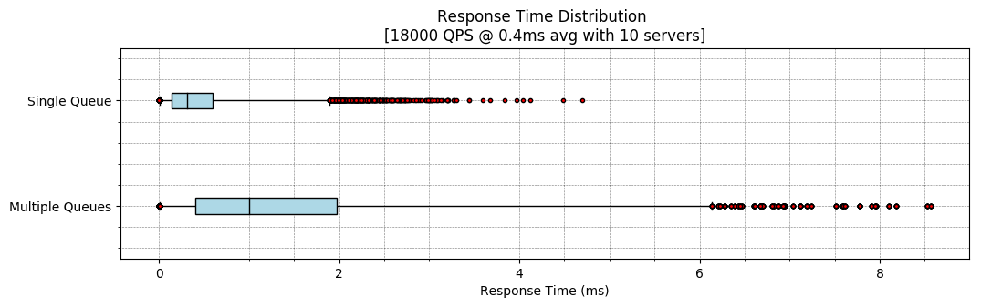
However, for reasonable request rates λ that do not put the system into an underloaded or overloaded state, we can see that the M/M/c queue dominates multiple queues using a jupyter notebook I wrote for helping me to simulate such queueing systems in high performance computing systems. For example if we simulate these two queueing systems using a 10 server farm with exponentially distributed service times with an average response latency of 0.4ms and a request rate of 18,000 requests per second (Poisson arrivals) we see that the multiple queues have about 300% the latency of a single queue across the latency distribution with significantly higher variance:

Theory:
E[T]_FDM = 1.43
E[T]_MMc = 0.44

Simulation:
Strategy         |    mean |     var |     p50 |     p95 |     p99 |   p99.9 |
Multiple Queues  |    1.41 |    1.83 |    1.00 |    4.11 |    6.13 |    7.96 |
Single Queue     |    0.43 |    0.17 |    0.31 |    1.25 |    1.89 |    2.86 |

We can also clearly see that a single queue is better by plotting the response latencies with a standard boxplot where the whiskers are placed at the 1st and 99th percentile latency:

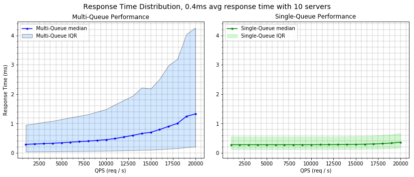
Alternatively we can look at the latency distribution of these two queueing options over a wide range of load and as we saw above the M/M/c continues to provide significantly better latency bounds:

Summary: Keeping work in a single queue is probably the right default choice if your goal is to minimize mean latency (maximize throughput).

Lesson #2: Balance your Load

It is fair to note that shoppers don’t just show up at one queue or the other, indeed they follow some form of algorithm where they try to select the best queue to join. In systems engineering we call this “load balancing” and we can improve immensely on the abysmal FDM results from above by using a smarter load balancing algorithm.

Load balancing happens when an external process intentionally picks the queue that a new request (customer) should enter to try to balance the load, it looks something like:

Load Balancing

We can explore three likely load balancing algorithms that customers in a grocery store may use in addition to our two strategies from above:

1. Random. The request is dispatched to a random worker. This should be equivalent to multiple queues from above.
2. Join Shortest Queue (JSQ): The request is dispatched to the worker with the shortest queue. This is a dynamic queueing policy as the load balancer makes a decision dynamically based on the queue state. This simulates when a customer scans every queue before checking out.
3. Best of Two Adjacent: This is a variant of the classic “choice of two” load balancing algorithm except that instead of picking any random two queues this one picks a random queue and picks between that queue and the one directly to the right and directly to the left. This simulates arriving at a random queue but then checking the queues to either side.

If we simulate these three options we can see that, again, the single queue dominates the field, although Join Shortest Queue is only very slightly worse (about 10% worse across the latency distribution).

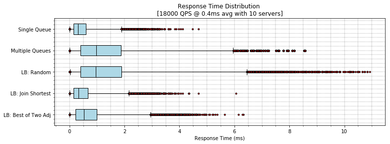
The surprise winner here in my opinion is the choice of two option, which underperforms JSQ but not by much, and unlike this simulation scanning all of the queues at the supermarket is not free. A good load balancing algorithm which is also lazy!? yes please.

We have seen that when we have to split into multiple queues, balancing the load really does help. This applies equally to computer systems: if you temporarily have more work to do then you have workers to do it, try to keep the work in a single queue as long as possible. When you do dispatch your work try to dispatch it to a worker that is free. For example if you’re running a website try to give a request to a web machine that has a free web worker right now. If you can’t do that, then try to have a good load balancer that get’s as close to that as possible.

Summary: If you must join a separate queue, try to go to the one with the least queued work. Joining the shortest queue you can is a good approximation of this (although as we will see in Part 2, estimating queued work is not exactly the same as the shortest queue).

Lesson #3: When you have picked the wrong queue, cheat

Unfortunately for you and me, supermarkets frequently choose the wrong way to queue their customers with individual queues per register. Computer programs also often don’t know how large the queues are at various destination servers or on various cores. The bright news is that there is a great technique we can borrow from high performance distributed systems: tied requests (aka request speculation).

With speculative/tied requests we as the customer try to get the fastest service time by dispatching to two or more workers, and you take whichever gets there first. Crucially to be efficient we have to drop the redundant request when the first starts being processed, however, we can still get a nice latency improvement even without this cancellation as shown in [2].

If we do a simulation of such tied requests where we always speculate and cancel the other request that is pending, we can see that tail latency is reduced dramatically:

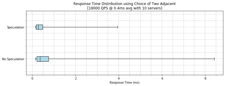
This is just like in a supermarket where a couple will split up and have one person wait at one register and the second person waits at a different register. Whoever gets to the cashier first tries to signal to the other person “hey come over here we can check out together” and they succeed at reducing their latency with no real decrease to throughput, although your fellow customers may be peeved at the surprise arrival of a potentially larger order.

Summary: In case you pick the wrong queue, you can just pick more than one queue and go to the one that dequeues first.

Conclusion

We’ve seen how supermarkets and high performance software services actually have a lot in common. Along the way we have hopefully learned how both queueing systems can take advantage of basic performance practices:

1. Use a smaller number of queues when you are worker bound that dispatch to free workers rather than having a queue per worker. This will likely increase throughput and decrease mean latency.
2. If you must balance between queues, choose something better than random load balancing. Ideally join queues with the closest approximation to shortest remaining work.
3. When you have multiple queues of unknown duration and latency is crucial, dispatch to multiple queues and race them against each other to get minimal latency.

Perhaps someday more supermarkets will see the light of better queueing theory and I’ll have less time to think about how I’m wasting time needlessly in line waiting to checkout.

Check out Part 2 for a slightly more sophisticated analysis.

Citations

[1] M. Harchol-Balter, Performance Modeling and Design of Computer Systems: Queueing Theory in Action. (google books)

[2] Jeffrey Dean and Luiz Andre Barroso, The Tail at Scale (paper)